Why accurate solar forecasting requires more than predicting sunlight

When people talk about solar forecasting, two terms are often used as though they mean the same thing: solar irradiance and solar generation. Although the two are closely connected, they describe fundamentally different parts of the solar energy conversion process. Solar irradiance represents the amount of solar radiation reaching a particular surface, while solar generation represents the amount of electrical energy that a photovoltaic plant can actually produce from that available solar resource. Understanding this distinction is essential to understanding modern solar power forecasting, because accurately predicting sunlight does not automatically mean accurately predicting electricity generation.

A solar plant does not convert every watt of incoming solar radiation into electricity. Between the atmosphere and the electricity exported to the grid is a complex chain involving cloud conditions, atmospheric characteristics, solar position, panel orientation, module temperature, photovoltaic conversion efficiency, inverter behaviour, system losses, plant availability and grid restrictions. As a result, an accurate solar generation forecast requires much more than a prediction of how sunny a particular location will be. It requires a model that can translate changing atmospheric conditions into the expected electrical response of a specific photovoltaic asset.

The fundamental forecasting chain can therefore be understood as atmospheric conditions → solar irradiance → irradiance on the PV array → DC electricity → AC electricity → grid export. Each stage introduces another layer of complexity, and errors introduced at one stage can propagate through the entire forecasting process. This is why plant-level photovoltaic power forecasting is fundamentally different from simply predicting solar irradiance.

THE FUNDAMENTAL DIFFERENCE

Solar Irradiance

Sun → Atmosphere → Clouds → GHI/DNI/DHI → W/m²

Solar Generation

Irradiance → Solar geometry → PV modules → Temperature effects → DC power → Inverter → AC power → Grid export → MW

Irradiance is the resource. Generation is the electrical response.

Solar Irradiance Is the Beginning, Not the Final Forecast

Solar irradiance is a measure of solar power received per unit area and is generally expressed in watts per square metre, or W/m². If a measurement indicates that global horizontal irradiance is 800 W/m², it means that approximately 800 watts of solar radiation are arriving at each square metre of a horizontal surface under those conditions. This measurement provides critical information about the available solar resource, but it does not directly tell us how much electricity a photovoltaic plant will generate.

Solar generation, on the other hand, is the electrical output of the PV system and is generally expressed in kilowatts or megawatts. A utility-scale solar plant may be producing 80 MW at a particular moment, but that number depends not only on the irradiance reaching the site but also on how the plant is configured and how its equipment responds to those conditions.

Consider two solar farms located relatively close to one another and experiencing broadly similar weather conditions. Both plants could receive a global horizontal irradiance of 700 W/m², yet their electrical output could be different. One plant may use fixed-tilt modules while the other uses single-axis trackers. One may have a DC capacity of 120 MW connected to 100 MW of AC inverter capacity, while another may have a different DC/AC ratio. Their module technologies, inverter efficiencies, temperatures, availability and system losses may also differ. The result is that the same atmospheric conditions can produce different electrical outputs.

This is the fundamental reason why accurate solar generation forecasting requires the model to understand the plant itself rather than simply the weather surrounding it.

Understanding the Different Types of Solar Irradiance

To understand why solar forecasting becomes increasingly complex as it moves from atmospheric conditions to electrical generation, it is important to distinguish between the major forms of irradiance used in photovoltaic modelling. Global Horizontal Irradiance, commonly referred to as GHI, represents the total solar radiation received on a horizontal surface. It consists of both direct radiation arriving from the sun and diffuse radiation scattered through the atmosphere.

Direct Normal Irradiance, or DNI, represents the direct solar radiation arriving from the direction of the sun on a surface positioned perpendicular to the incoming solar rays. Diffuse Horizontal Irradiance, or DHI, represents radiation that has been scattered by molecules, aerosols and clouds before reaching a horizontal surface. Conceptually, GHI can be expressed as the combination of diffuse radiation and the horizontal component of direct radiation, represented by the relationship GHI = DHI + DNI × cos(θz), where θz is the solar zenith angle.

These distinctions become important because photovoltaic modules are not normally installed horizontally. They have a particular tilt and azimuth, and many utility-scale installations use tracking systems that continuously change their orientation relative to the sun. Consequently, the amount of radiation arriving on the module surface can differ significantly from the GHI measured or forecast for the location.

This leads to another important variable: Plane-of-Array irradiance, commonly called POA irradiance. POA represents the solar radiation incident on the actual surface of the photovoltaic array. NREL's System Advisor Model documentation distinguishes GHI, DNI and DHI and uses solar geometry and array orientation to calculate the irradiance incident on the PV array.

For a solar generation forecasting system, this transformation is critical. The PV modules do not generate electricity directly from an abstract number representing horizontal irradiance. They respond to the radiation actually reaching their surfaces.

FROM GHI TO POA

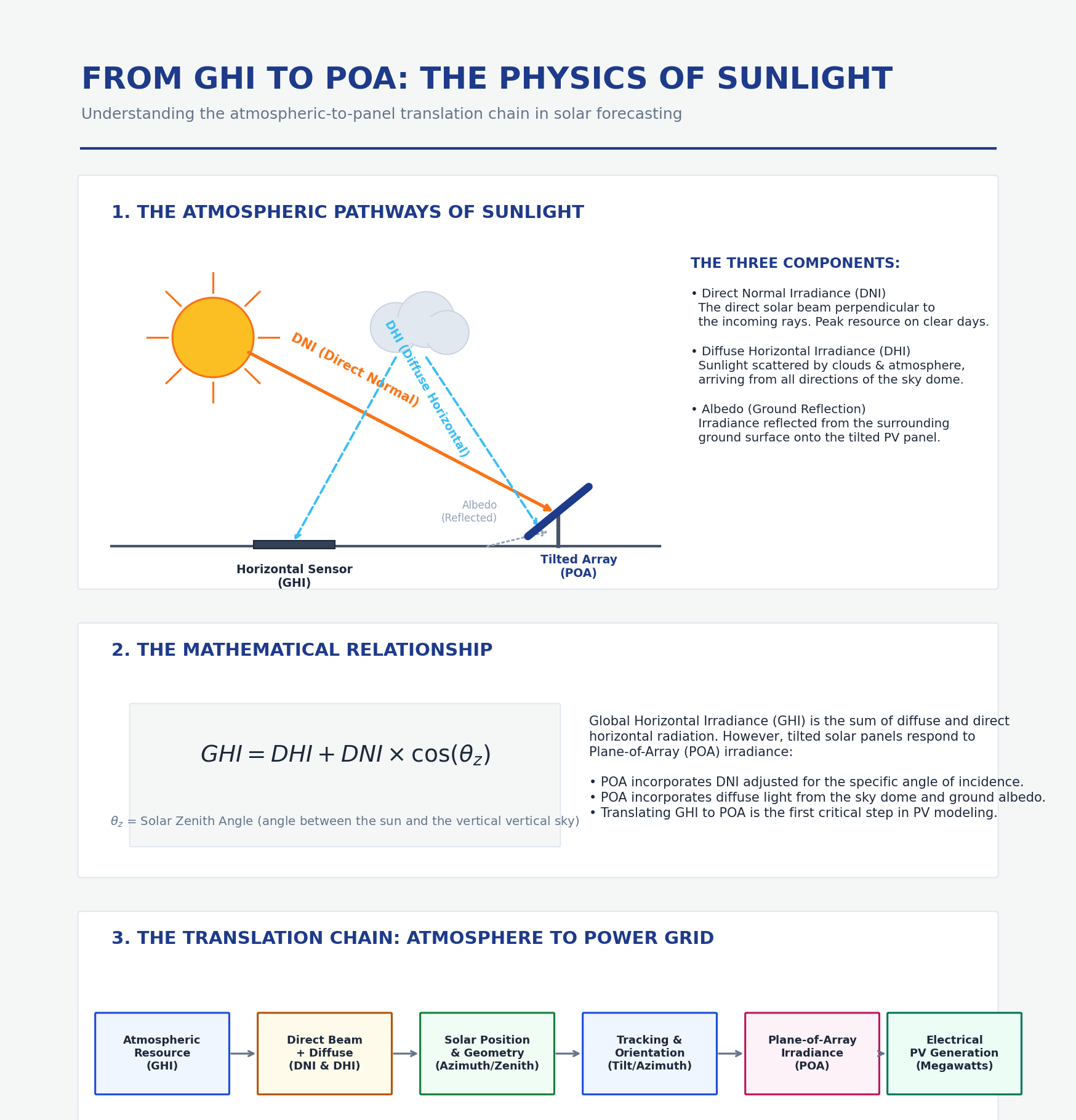
A technical illustration showing the sun above a solar panel with three radiation paths. One arrow should represent direct radiation from the sun to the panel, another should represent diffuse radiation from the sky, and another should represent reflected radiation from the ground. The diagram should then show GHI → DNI + DHI → Solar Position → Panel Tilt → Panel Azimuth → Tracking Position → POA Irradiance.

The key message should read:

The PV plant does not generate electricity from GHI directly. It responds to the irradiance actually reaching the PV array.

Clouds Make Solar Irradiance Difficult to Forecast

The amount of solar radiation reaching a solar plant changes continuously as atmospheric conditions evolve. Some of this variation is relatively predictable. Solar position follows a well-defined astronomical pattern, meaning that the approximate movement of the sun and the clear-sky component of irradiance can be calculated with considerable precision.

Clouds are much more complicated.

A cloud system can form, grow, move, merge with another cloud system, dissipate or change its optical characteristics over a relatively short period. This creates rapid changes in the amount of radiation reaching the ground. A solar plant operating under clear skies may suddenly experience a major reduction in irradiance when a dense cloud formation passes overhead. Once the cloud moves away, generation may recover rapidly.

This creates what the solar industry commonly refers to as a ramp event. A large photovoltaic plant could be producing 90 MW at one moment and significantly less only a short time later because of cloud movement. From the perspective of a grid operator or energy trader, knowing that the day will be “partly cloudy” is not enough. The important information is when the cloud will reach the plant, how much irradiance it will block and how the plant will respond to that change.

This is one of the reasons satellite-based solar irradiance forecasting has become increasingly important for short-term forecasting. Satellite imagery provides a spatial view of cloud fields rather than simply measuring the atmospheric conditions directly above one point. Research into satellite-based solar forecasting has demonstrated the value of cloud movement information for short-term irradiance prediction, particularly when rapidly changing cloud fields create significant variability.

THE MOVING-CLOUD PROBLEM

The infographic should show a solar plant from a top-down perspective with a cloud formation approaching from the west. At the first timestamp, the cloud should be approximately 25 kilometres away. At the next timestamp, it should be closer to the plant. The third image should show the cloud partially covering the plant, followed by a fourth image showing the cloud covering most of the plant and a fifth showing the cloud moving away.

Below the satellite-style sequence, show two curves representing irradiance and PV generation.

The headline should be:

A solar forecast is not just about whether clouds exist. It is about where those clouds will be when they reach the plant.

Cloud Motion Turns Satellite Images Into Forecast Information

A satellite image tells us what the atmosphere looks like at a particular moment. Forecasting requires us to estimate what that atmosphere will look like in the future. This is where Cloud Motion Vectors, or CMVs, become important.

A Cloud Motion Vector represents the apparent movement of a cloud feature between two observations. If a recognisable cloud structure moves a certain distance between two satellite images, its displacement can be used to estimate its direction and velocity. Conceptually, velocity can be expressed as displacement divided by time.

For example, if a cloud structure moves 10 kilometres eastward in ten minutes, its approximate movement is 60 kilometres per hour. If the observed trajectory remains reasonably consistent, the forecasting system can project where the cloud may be located in the future. That projected cloud position can then be related to the geographic location of a solar plant.

This is a major conceptual shift in solar forecasting. Instead of simply asking what the weather is like at the plant right now, the forecasting system can consider what atmospheric structures are moving toward the plant and how they may affect future irradiance.

HelioExpect's forecasting architecture uses high-resolution satellite imagery and cloud-motion analysis to identify cloud movement and estimate how approaching cloud structures may influence solar irradiance at a plant.

WHAT A CLOUD MOTION VECTOR ACTUALLY DOES

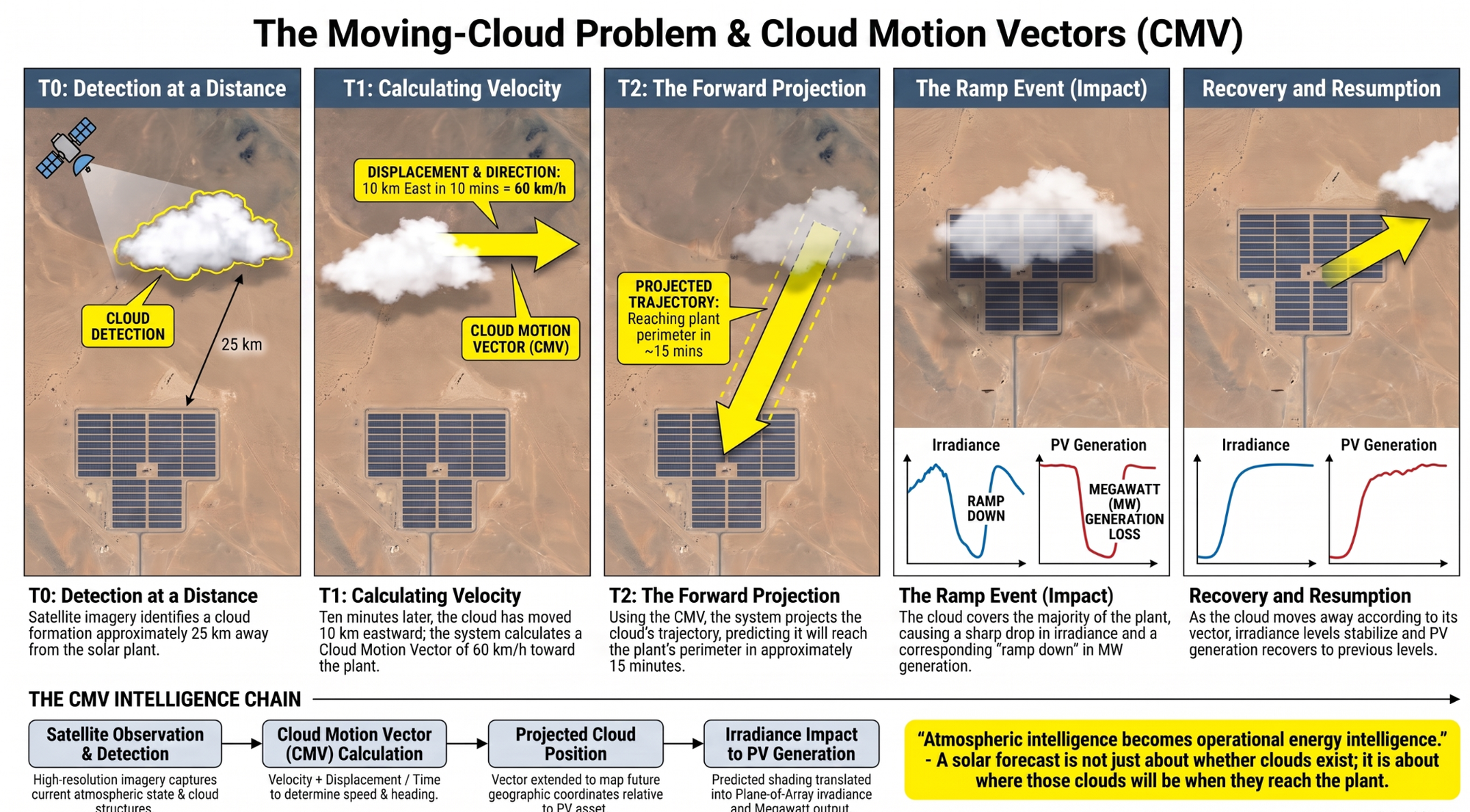
The graphic should show a cloud feature at T0 and the same feature at T1. An arrow should connect the two positions and be labelled with its displacement and direction. A second arrow should extend forward to show the projected position at T2.

The diagram should then connect the projected cloud position to the solar plant.

Satellite Observation → Cloud Detection → Cloud Motion Vector → Projected Cloud Position → Irradiance Impact → PV Generation

The Advantage of Seeing Beyond the Solar Plant

A ground-based irradiance sensor is extremely valuable because it provides a direct measurement of current conditions at the site. However, it primarily answers one question: what is happening here right now?

A satellite image can help answer a different question: what is happening around the plant and what may reach the plant next?

Imagine a solar plant currently experiencing nearly clear conditions with a measured GHI of 950 W/m². A sensor at the plant may indicate that generation conditions are excellent. At the same time, satellite imagery may show a large cloud formation 15 kilometres away moving directly toward the plant.

A forecasting system that relies heavily on current conditions might assume that the present state will continue. A cloud-aware system can instead incorporate the incoming cloud structure into its short-term forecast.

This distinction is particularly important for solar nowcasting, where the objective is to forecast conditions over relatively short time horizons. The closer the forecast horizon is to the present, the more valuable information about the current spatial structure and movement of clouds can become.

From Irradiance to Electrical Power

Once the future irradiance has been estimated, the forecasting problem is still not finished.

The model now needs to convert irradiance into electrical power.

At a simplified level, the transformation can be represented as:

Irradiance → PV cell response → DC power → Inverter → AC power → Grid export

However, every stage of this process contains additional variables.

Photovoltaic modules have electrical characteristics that determine how they respond to incident irradiance. Their performance also changes with temperature. As module temperature increases, the electrical efficiency of conventional PV technologies generally decreases. This means that two periods with similar irradiance can still produce different electrical outputs if the module temperatures are different.

Temperature therefore becomes an important input to accurate photovoltaic power forecasting. A forecasting system needs to understand the relationship between incoming solar radiation, environmental temperature and the electrical response of the PV modules.

The Role of Panel Orientation and Tracking

The physical orientation of the photovoltaic array introduces another layer of complexity. A fixed-tilt PV plant maintains a relatively stable orientation throughout the day, while a single-axis tracking system changes its orientation according to the position of the sun.

The same weather conditions can therefore produce different POA irradiance at two plants.

Consider two identical solar modules located at the same site. If one module is mounted on a fixed structure and another is mounted on a tracker, the angle at which sunlight strikes the two surfaces will differ throughout the day. Consequently, their effective irradiance and electrical output can also differ.

At utility scale, these differences become significant. A solar generation forecasting system must understand the physical configuration of the plant if it is expected to predict electrical output rather than simply atmospheric conditions.

SAME WEATHER, DIFFERENT GENERATION

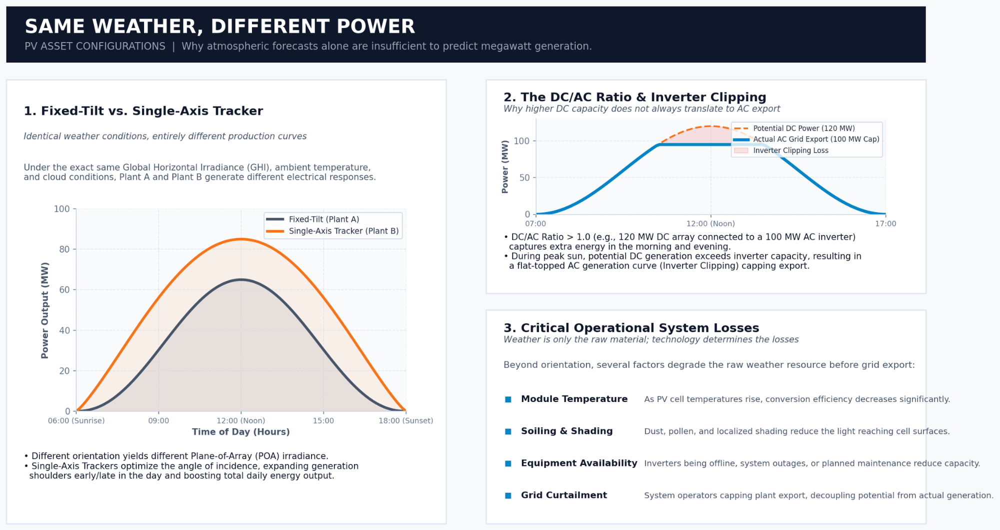
Show two solar plants experiencing exactly the same weather.

PLANT A: Fixed tilt

PLANT B: Single-axis tracker

Above both plants:

Same GHI | Same Temperature | Same Cloud Conditions

Then show:

Different orientation → Different POA → Different electrical output

The sky can be the same while the power output is different.

Why the DC/AC Ratio Matters

Another important factor is the relationship between the DC capacity of the PV modules and the AC capacity of the inverters. Utility-scale solar projects frequently install more DC capacity than the nominal AC capacity of their inverters. For example, a project could have 120 MW of DC capacity connected to 100 MW of AC capacity.

This configuration allows the plant to capture more energy during periods when irradiance is below the level required to reach maximum inverter output. However, during periods of very high irradiance, the DC array may theoretically be capable of producing more power than the inverter can convert into AC electricity.

The result is inverter clipping.

This means that even if a forecasting system predicts very high irradiance, the plant may not continue increasing its AC output indefinitely. Once the inverter reaches its operating limit, additional available DC power cannot translate directly into additional AC generation.

Consequently, the DC/AC ratio is an important component of plant-level photovoltaic power modelling.

Solar Generation Is Also Affected by System Losses

Between the available solar resource and electricity delivered to the grid, energy can be lost at multiple stages. The magnitude of these losses depends on the characteristics and operating condition of the individual plant.

Soiling can reduce the amount of radiation reaching the modules. Shading can reduce output from affected sections of the array. Module temperature can reduce conversion efficiency. Electrical resistance can introduce DC-side losses. Inverters have their own efficiency curves, while transformers and other electrical equipment introduce additional losses.

Plant availability can create another difference between theoretical and actual generation. A PV model may determine that a plant should be capable of generating a particular amount of electricity under given conditions, but if an inverter block is offline, maintenance is underway or the grid is restricting output, actual generation can be lower.

Curtailment is particularly important because it creates a distinction between the power the plant could have generated and the power it was actually permitted to export.

For an operational solar forecasting system, this distinction matters enormously.

The objective is not simply to estimate the theoretical output of the PV modules. It is to estimate the generation that is relevant to the operational environment.

Why Historical SCADA Data Matters

This is where plant-specific historical data becomes particularly powerful.

A theoretical PV model can describe how a solar plant should behave under particular physical conditions. But real plants rarely behave exactly like ideal mathematical systems.

Over time, operational data reveals the actual behaviour of the asset.

SCADA systems can provide historical information about generation, irradiance, temperature, inverter performance and other operational variables. When forecast values are continuously compared against actual plant behaviour, systematic differences can become visible.

For example, if a model consistently predicts 85 MW while the plant repeatedly produces approximately 80 MW under comparable conditions, the difference may represent a systematic bias. It could be related to soiling, plant configuration, equipment behaviour, temperature response, sensor characteristics or another site-specific factor.

Machine learning can be used to identify these patterns and correct the forecast.

The process therefore becomes iterative:

Forecast → Actual generation → Forecast error → Learning → Bias correction → Improved forecast

HelioExpect describes this approach through plant-level modelling, SCADA history and machine-learning-based bias correction, with forecast performance continuously compared against actual generation.

THE SELF-CORRECTING FORECAST

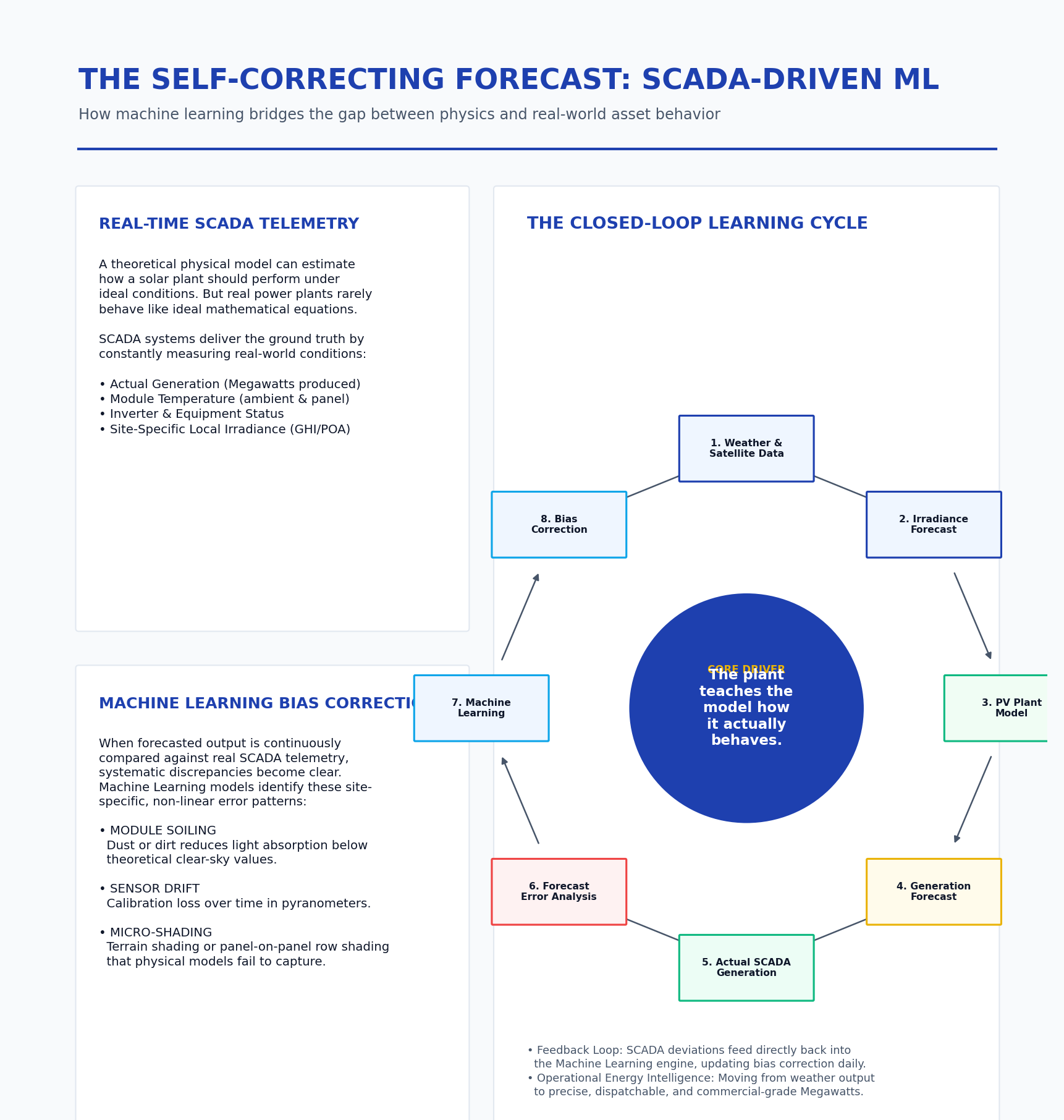
Create a circular technical diagram showing:

Weather & Satellite Data

↓

Irradiance Forecast

↓

PV Plant Model

↓

Generation Forecast

↓

Actual SCADA Generation

↓

Forecast Error

↓

Machine Learning

↓

Bias Correction

↓

Improved Generation Forecast

At the centre:

The plant teaches the model how it actually behaves.

Why a Weather Forecast Alone Is Not Enough

A weather forecast might say that tomorrow will be sunny with intermittent clouds. That information can be useful for general planning, but it is not sufficiently granular for a utility-scale solar operator managing hundreds of megawatts of generation.

An energy trader may need to know how much electricity will be available at a particular market interval. A grid operator may need to understand when generation could increase or decrease. An asset manager may need to determine whether a production deviation is caused by weather or equipment. A battery operator may need to decide when to charge or discharge storage.

All of these decisions require an electrical power forecast rather than a generic weather forecast.

This is why the most useful solar forecasting systems transform information through multiple layers. Atmospheric data is converted into irradiance information, irradiance is converted into expected PV output, and the resulting forecast is corrected using historical plant behaviour.

The ultimate objective is therefore not simply to predict the weather.

It is to predict the electrical response of the asset.

The Forecast Horizon Changes the Problem

Another reason solar forecasting cannot rely on a single data source is that the importance of different information changes with the forecast horizon.

A forecast for the next 15 minutes is fundamentally different from a forecast for tomorrow or the next seven days. For very short horizons, the current state and movement of clouds can be extremely important. Satellite imagery and Cloud Motion Vectors can provide information about cloud structures approaching the plant.

As the forecast horizon increases, atmospheric weather models become increasingly important because the forecasting problem shifts from extrapolating the current state toward predicting the future evolution of the atmosphere.

This is why advanced AI solar forecasting architectures increasingly combine multiple sources of information instead of attempting to use one model for every forecasting horizon.

HelioExpect describes a hybrid architecture combining satellite information, Cloud Motion Vectors, GraphCast-based weather modelling, plant-level modelling and machine-learning correction across different forecasting horizons.

THE SOLAR FORECASTING HORIZON

Create a horizontal timeline:

Now → 15 min → 1 hour → 3 hours → 24 hours → 7 days → 14 days

As the timeline progresses, visually show different sources becoming more prominent:

Satellite + CMV → AI/NWP → Plant Model → ML Correction → Long-range Weather Models

Headline:

Different horizons require different information.

From Cloud Movement to Megawatts

Consider a 200 MW solar PV plant producing 165 MW at 10:00 in the morning. Current irradiance is high and satellite observations indicate relatively clear conditions over the plant.

However, satellite imagery also identifies a large cloud formation approximately 30 kilometres to the west. The cloud structure is moving eastward at approximately 45 kilometres per hour.

The forecasting system can use the observed cloud trajectory to estimate when the cloud formation may reach the plant. It can then combine this information with solar position, predicted irradiance attenuation, plant configuration, temperature and historical plant behaviour.

Instead of simply assuming that current generation will continue, the system can generate a forecasted generation curve in which output increases initially as solar elevation rises and then decreases as the cloud structure affects the plant.

The important output is not simply an irradiance value.

It is the expected generation trajectory.

This is the difference between saying:

“A cloud is approaching.”

and saying:

“The plant is expected to experience a significant reduction in generation approximately 40 minutes from now.”

For energy operations, the second statement is considerably more useful.

FROM SATELLITE TO MEGAWATTS

Show a five-stage transformation:

01 — Satellite Image

↓

02 — Cloud Motion Vector

↓

03 — Future Irradiance

↓

04 — Plant-Specific PV Model

↓

05 — Expected MW Output

At the bottom:

Atmospheric intelligence becomes operational energy intelligence.

Why Forecast Accuracy Must Ultimately Be Measured at the Power Level

A forecasting system can achieve excellent irradiance prediction while still producing a poor generation forecast.

Suppose a model predicts 950 W/m² of irradiance and the actual irradiance is 940 W/m². On the surface, that may appear to be a relatively small error. But if the model has incorrect assumptions about module temperature, inverter availability, tracking behaviour, system losses or plant configuration, the resulting generation forecast could still be significantly wrong.

This is why serious photovoltaic power forecasting requires validation throughout the complete forecasting chain.

The system should be able to evaluate the quality of the weather inputs, the irradiance forecast and, ultimately, the electrical generation forecast against actual plant output.

The final question is therefore not simply:

How accurately did we predict the irradiance?

It is:

How accurately did we predict the electricity the plant actually generated?

Why This Matters for the Grid

Solar generation is variable, and large changes in photovoltaic output can create operational challenges as solar penetration increases.

When a cloud system passes over a large solar installation, generation can decline rapidly. When the cloud moves away, generation can recover just as quickly. If these changes are not accurately anticipated, grid operators may need to respond using other generation resources, reserves or storage.

Accurate solar power forecasting can therefore support generation scheduling, grid balancing, market participation, battery dispatch and deviation management.

Research into solar forecasting continues to emphasize its importance for grid balancing, electricity markets, storage management and renewable integration.

The practical objective of forecasting is therefore to transform uncertainty into something that can be managed.

The Future of Solar Forecasting Is Hybrid

The complexity of solar generation means that no single data source is sufficient for every forecasting problem.

Satellite imagery provides a spatial view of cloud fields. Ground sensors provide direct measurements of current conditions. Numerical Weather Prediction models provide atmospheric forecasts. Cloud Motion Vectors describe the movement of observed cloud structures. PV physics translates irradiance into expected electrical behaviour. SCADA data reveals how the actual plant performs. Machine learning can identify relationships and systematic errors that are difficult to capture through a purely physical model.

The future of AI solar forecasting is therefore unlikely to be about replacing one methodology with another.

Instead, it will involve combining complementary sources of information.

The architecture becomes:

Satellite observations + Cloud Motion Vectors + Weather Models + PV Physics + SCADA + Machine Learning

The strength of this approach lies in the fact that each component answers a different question.

Satellite imagery helps answer what is happening in the atmosphere.

Cloud Motion Vectors help answer where cloud structures are moving.

Weather models help answer how atmospheric conditions are likely to evolve.

PV physics helps answer how the plant should respond.

SCADA data helps answer how the plant actually behaves.

Machine learning helps bridge the gap between the expected and observed behaviour.

Together, these components create a much more complete representation of the solar generation problem.

From Weather Forecasting to Energy Intelligence

The evolution of solar forecasting can therefore be viewed as a progression.

The first question was:

What will the weather be?

The next question became:

How much solar radiation will reach the site?

The next question became:

How much electricity will the PV system generate?

The next generation asks something even more useful:

What will the plant generate, when will it generate it, how certain is that forecast, and what should the operator do with that information?

This final stage transforms forecasting from a weather service into an energy intelligence system.

The forecast can become an input into market bidding, generation scheduling, deviation management, battery dispatch, portfolio optimisation and operational planning.

That is ultimately why the difference between irradiance and generation matters.

Irradiance Is the Input. Generation Is the Outcome.

The difference between solar irradiance and solar generation may appear simple, but it is fundamental to accurate photovoltaic power forecasting.

Irradiance tells us how much solar energy is available.

Generation tells us how much electricity a particular solar plant can actually produce.

Between those two points is an entire chain of atmospheric science, satellite observation, cloud tracking, solar geometry, photovoltaic physics, equipment modelling, historical SCADA analysis and machine learning.

A modern solar generation forecast therefore cannot stop at predicting sunlight.

It must understand the atmosphere, determine how clouds are moving, estimate the irradiance that will reach the PV array, model how the plant will respond to that irradiance and continuously compare its predictions with what the plant actually produces.

The distinction becomes particularly important as solar penetration increases and grid operators require increasingly precise information about renewable generation.

The future of solar forecasting is therefore not simply about predicting whether tomorrow will be sunny.

It is about building a continuous bridge between the atmosphere and the power grid.

Satellite observations reveal what is happening above the plant.

Cloud Motion Vectors help estimate what is moving toward it.

Weather models provide a view of how the atmosphere may evolve.

PV models translate irradiance into electrical response.

SCADA data reveals how the asset actually behaves.

Machine learning learns from the difference.

And the final output is not measured in watts per square metre.

It is measured in:

Megawatts.

Because solar operators do not ultimately need to know how much sunlight is in the sky.

They need to know:

How much power will this solar plant actually deliver and when?

That is the fundamental problem modern solar generation forecasting must solve.